The discovery of penicillin (which we talked about in our previous installment) contributed to the birth of the new field of antibacterial medicine. However, infectious diseases were not the only scourge of the 20th century. At the beginning of the century, the study of hereditary diseases began gaining popularity. This trend would mark the beginning of the study of genomes, which would be decoded primarily with the help of another revolutionary 20th century invention: computers.
By the middle of the century, the computational capabilities of computers and a deep theoretical understanding of the processes occurring at the cellular level would allow humanity to decipher the secrets of the genome, and by the end of the century – to clone the first mammals.
Unraveling the mystery of the genome
The first ideas about hereditary diseases were formulated by English physician Archibald Garrod in the early 20th century. In his 1902 paper entitled “The Incidence of Alkaptonuria: A Study of Chemical Identity” he defines “chemical individuality” as a person’s genetic predisposition to certain hereditary diseases. Archibald Garrod understood that the information that shapes us must be stored at the cellular level, transmitted hereditarily, and follow a number of chemical and biological patterns.
And although Garrod was a great innovator who predicted the existence of the genome 40 years before its actual discovery, he was not the first to think about the genetic inheritance inherent in biological species. Works on the theory of evolution by Charles Darwin (who put forward the idea of pangenesis) and the Augustinian monk Gregor Mendel, who studied heredity in plants (“Experiments on Plant Hybridization,” 1865) in the 19th century would lay a reliable foundation for the further formation of genetics as a full-fledged science. It was only a question of when science would be able to prove the hypotheses they had put forward.
In 1911, the American zoologist and geneticist Thomas Morgan, observing the ability of Drosophila flies to genetically inherit eye color, came to the conclusion that genetic information should be contained in chromosomes – nucleoprotein structures located in the nucleus of a eukaryotic cell.
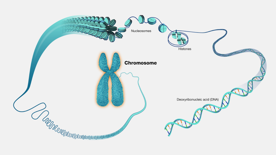
Chromosomes are constructed from proteins and thread-like molecules of deoxyribonucleic acid (DNA), and until the middle of the century, scientists studying genetics could not figure out exactly where a cell’s genetic information was supposed to be stored. A 1944 experiment by three American geneticists (Oswald Avery, Colin Macleod, and Maclyn McCarty) resolved this issue. After conducting research on mice and introducing them to dead pneumococcal bacteria, scientists proved that it is the DNA molecule (and not the protein) that contained the primary information about the strains of these bacteria. Proteins enclosed in chromosomes were also endowed with their own function – they were responsible for the process of DNA replication and the expression of one or another type of heredity in it.
Their 1944 article in the Journal of Experimental Medicine turned the scientific world upside down. More and more scientists would begin studying chromosomes.
In the middle of the century, it would become clear that the number of chromosomes in the nucleus of living organisms varied by species: for example, a human cell stores 23 pairs of chromosomes: 22 autosomes and 1 pair of sex chromosomes (XX or XY). Each offspring inherits an equal number of chromosome pairs from their parents, which is why we are equally similar to both of our parents.
In 1953, thanks to the work of James D. Watson and Francis Crick, we learned that human DNA is a double helix molecule resembling a ladder, with nitrogenous bases forming the steps between the two sides. In total, there are 4 of these nitrogenous bases:
- A – adenine, a nitrogenous base forming 2 hydrogen bonds with uracil and thymine.
- C – cytosine, a nitrogenous base forming 3 hydrogen bonds with guanine.
- G – guanine, a nitrogenous base that forms 3 hydrogen bonds with cytosine and is an integral part of nucleic acids.
- T – thymine, a nitrogenous base, one of the functions of which is to scatter ultraviolet radiation and protect the DNA molecule from the effects of solar radiation.
Put simply, the sequence of these nitrogenous bases created the formula by which this or that species was formed. It is these sequences that make us and every other living organism who we are. Watson and Crick published their paper on this discovery, entitled The Molecular Structure of Nucleic Acids: A Structure for Deoxyribonucleic Acid, in the journal Nature on April 25, 1953. The ladder structure of DNA perfectly explained its mechanism of replication. Today, we know that the sequence of the human DNA chain consists of more than 3300 million base pairs.
In the second half of the 20th century, the scientific community took on the challenge of deciphering the DNA structure of other organisms, trying to understand their genetic sequences. The decoding process would theoretically give scientists the opportunity to intervene in the very process of creating life, producing new types of genetically-modified organisms.
Unraveling the mystery of the genome would launch the new science of molecular biology, which would allow scientists to make modifications to DNA, and thereby create new types of genetically modified crops. By the end of the century, in 1996, scientists would even clone the first mammal: a sheep named Dolly.
Prior to the Dolly cloning experiment by the team of the Scottish Roslin Institute’s Ian Wilmut, geneticists believed that DNA molecules differed between different cells of the same organism. Thus, it was erroneously believed that the DNA in a kidney cell would contain information about the work of the kidneys and, therefore, differ from the DNA located in a brain cell. Ian Wilmut was sure this was not the case. He cloned Dolly with just one mammary cell from the original sheep.
After confirming that the cloned sheep embryo did not contain any pathologies, it was transplanted into another sheep, which acted as Dolly’s surrogate mother. Born on July 5, 1996, the sheep was genetically identical to its original. Despite the fact that the cloned Dolly was born in 1996, the world community learned about her appearance only a year later, after Professor Wilmut published his research.
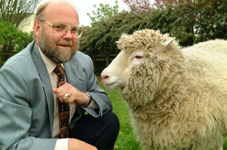
Photo courtesy of the Roslin Institute, University of Edinburgh, UK.
It is worth noting that such breakthroughs in genetic engineering would not have been possible without the power of computers, which scientists had been actively developing in the second half of the 20th century. These computing machines were able not only to determine the sequence of the genome, but also to create amazingly complex computer models, significantly increasing our capacity to make scientific predictions.
The Dawn of Computing Machines: The First Generation of Computers
Mechanical computers have been known since the 17th century, when French mathematician Blaise Pascal created his arithmetic machine, but the first fully electronic computers began to appear only in the 1940s.
The first model of an electronic computer appeared in Germany in 1941. Its inventor was the German engineer Konrad Zuse. The model, which he would call Z3, was a fully programmable electronic computer that could work with binary code. The computer was used in calculations to create more advanced wings and fuselages for aircraft, and later the bodies of the first German V2 ballistic missiles. The only Z3 machine in existence was destroyed during an Allied air raid on Berlin in 1945.
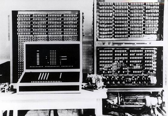
Photo: Konrad Zuse Internet Archive/Deutsches Museum/DFG
Konrad Zuse’s computer was the successor of the two machines he had developed earlier, the Z1 and Z2. Input parameters were applied using punched cards – thick pieces of cardboard with specially-placed holes. Zuse’s computers were equipped with instructions for reading information from punched cards, which is how they received their instructions, after which the calculation process started.
Zuse was surprisingly accurate in identifying the principles by which computer technology would work in the foreseeable future:
- A binary number system.
- Machine logic – operating with the categories “yes / no.”
- A fully-automated calculation procedure.
- Programmability – The operator of the machine specifies the input parameters and the task that the computer must perform
- Using high-capacity memory.
- Support for moving point arithmetic
Konrad Zuse would survive World War II and in 1950 release his next computer model, the Z4. In addition to being the first computer to be commercially sold, the Z4 was also the first computer to use a high-level programming language, which Zuse called Plankalkül (translated from German as “calculation plan”).
In 1945, at the University of Pennsylvania with the help of physicist John W. Mauchly and engineer J. Presper Eckert, the first American computer was built, called the ENIAC (Electrical Numerical Integrator and Calculator).
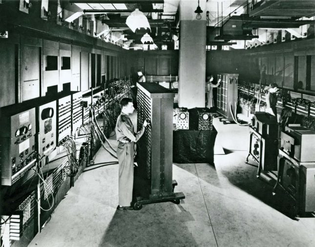
The ENIAC was developed during the Second World War, and its main task was to calculate range tables to correct artillery fire. The computer used vacuum tubes as the main components of its processor and memory. The weakest component of the ENIAC was a mechanical system for reading commands using punched cards prepared by the machine’s attendants. This technology could not keep up with the computational work of a computer in any way, as it took several days to retrain the machine to execute a new type of instruction.
American computers largely worked on computational algorithms created by the English mathematician Alan Turing, which he implemented in his 1936 idea of a universal Turing machine. The Universal Turing Machine (which the scientist himself called “Automaton” or a-Machine) was an abstract idea of a computer capable of producing a mathematical model of computation. Conceptually, the Turing machine was an analogue of the modern CPU (central processing unit) responsible for performing computational operations in a computer. For its memory, the machine used a tape segmented by cells, which contained a set of commands (analogous to modern programming code).
It is important to understand that the machine itself did not exist as a physical object, but was rather simply an idea of how to make a computer perform the actions required of it. Turing was one of the first to describe algorithms for this machine logic.
Computers like the American ENIAC, the Z3, and the UNIVAC-1 and EDVAC which followed them are considered to be first-generation computers. They were slow, bulky, and in need of continuous maintenance by a large number of highly-qualified personnel. However, it was already clear during the time of these machines that the first transistorized computers were on the horizon.
The next generations of computers
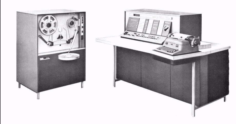
The second generation of computers (produced mainly from 1957 to 1963) worked on transistors. Transistors, which were more compact and cheaper, replaced electronic vacuum tubes, allowing the new machines to significantly increase their computing power while also reducing their size. Now, the computers no longer needed to occupy an entire room, but instead could match their predecessors while occupying only a few square meters. Second-generation computers would enter commercial markets, making them far more accessible to designers and engineers. The automation of calculations and accounting would move to a qualitatively new level in these years and would give a much-needed impetus to the growth of American industry.
The second generation of computers also brought the emergence of high-level programming languages, the most popular of which were Fortran and Cobol. The primary memory in transistor computers was implemented as a magnetic core, and the recorded results of calculations could be stored on the first computer diskettes and magnetic tapes. In addition, the first data input devices appeared, which took the form of a typewriter.
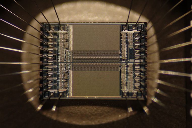
The era of third-generation computers would begin in 1964 and last until 1971. These machines would completely replace transistors with integrated circuits (ICs) – electronic circuits made on a semiconductor substrate, most often silicon chips. This technology made it possible to fit tens of thousands of bits of data on a chip the size of a palm, as well as provide a fast data transfer rate, since now all the transistors were located on a single small chip, and the movement of electrons took much less time. It is in third-generation computers that the first operating systems would appear.
Semiconductor chips would shape the look of the computer as we know it today. Computers of the fourth (1971-1980) and fifth generations (from 1980 to the present day) will still work on integrated circuits, and the main difference between them is only a decrease in the size of microprocessors and, as a result, an increase in their computing power.
However, even the most modern computer technology today faces an impenetrable ceiling, which is that all computers known today operate with bits (0 and 1). As a result, even the most powerful of them will always process information in a strictly linear way. When performing 100 different operations, each of them is performed sequentially, which significantly increases the time required to complete complex multi-tasking program cycles.
The situation is sure to be changed by quantum computers, which are already being developed today. Quantum computers will operate on qubits (in which the values 1 and 0 are taken simultaneously), which will allow these machines to process all possible states simultaneously and endow it with the property of multitasking, in the full sense of the word. But before this can be realized, people will first need to significantly expand their understanding of quantum theory.